Programming Assignment #2 15-463: Rendering and Image Processing

IMAGE WARPING and MOSAICING

Due Date: by 11:59pm, Th, Oct 7
Milestone Due Date: Th Sept 30

The goal of this assignment is to get your hands dirty in different aspects of image warping with a “cool” application -- image mosaicing. You will take two or more photographs and create an image mosaic by registering, projective warping, resampling, and compositing them. Along the way, you will learn how to compute homographies, and how to use them to warp images. As background for this assignment, read Projective Mappings for Image Warping notes by Paul Heckbert, and Image Alignment and Photo Stitching Tutorial (DRAFT) by Richard Szeliski.

The core of the assignment should be done individually. However, major data acquisition tasks as well as the Bells & Whistles can be done in pairs.

The steps of the assignment are:

1. Shoot and digitize pictures (20 pts)
2. Recover homographies (25 pts)
3. Warp the images (20 pts)
4. Blend images into a mosaic (20 pts)
5. Submit your results

In addition, there will is a number of extra Bells & Whistles that extend this project in various ways. You will need to do at least some of them to get full credit. Anything above 100 points will be counted as extra credit.

In the latest version of Matlab, there are some functions that are able to do much of what is needed. However, we want you to write your own code. Therefore, you are not allowed to use the following functions in your solution: cp2tform, imtransform, tformarray, tformfwd, tforminv, and maketform. On the other hand, Matlab has a number of very helpful functions (e.g. for solving linear systems, inverting matrices, linear interpolation, etc) that you are welcome to use. If there is a question whether a particular function is allowed, ask us.

WARNING: This assignment will take some time and effort. Start early and good luck!

Shoot the Pictures

Shoot two or more photographs so that the transforms between them are projective (a.k.a. perspective). One way to do this is to shoot from the same point of view but with different view directions, and with overlapping fields of view. Another way to do this is to shoot pictures of a planar surface (e.g. a wall) or a very far away scene (i.e. plane at infinity) from different points of view.

The easiest way to acquire pictures is using a digital camera. We have two Canon A60s to lend (talk to James). Make sure to use the highest resolution setting (important for homography calculation; you can always downsample it later). There will be a universal media card reader installed in the graphics cluster which you can use to download the images into your account. Matlab’s imread can take most popular image formats; use unix convert for the more obscure ones.

While we expect you to acquire most of the data yourself, you are free to supplement it with other sources (old photographs, scanned images, the Internet). We're not particular about how you take your pictures or get them into the computer, but we recommend:

• Avoid fisheye lenses or lenses with significant barrel distortion (do straight lines come out straight?). Any focal length is ok in principle, but wide angle lenses often make more interesting mosaics.
• Shoot as close together in time as possible, so your subjects don't move on you, and lighting doesn't change too much (unless you want this effect for artistic reasons).
• Use identical aperture & exposure time, if possible. On most "idiot cameras" you don't have control of this, unfortunately. It's nice to use identical exposures so that the images will have identical brightness in the overlap region.
• Overlap the fields of view significantly. 40% to 70% overlap is recommended. Too little overlap makes registration harder.
• It's OK to vary the zoom between pictures.
• If you're shooting a non-planar scene, then shoot pictures from the same position (turn camera, but don't translate it). A tripod can help in this, particularly if objects are close.

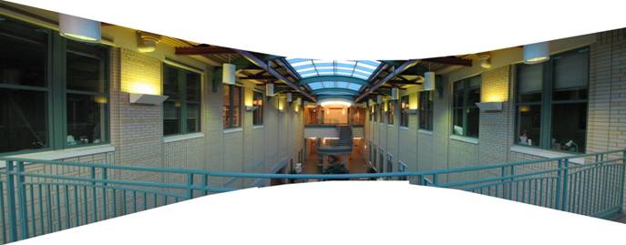
Good scenes are: building interiors with lots of detail, inside a canyon or forest, tall waterfalls, panoramas. The mosaic can extend horizontally, vertically, or can tile a sphere. You might want to shoot several such image sets and choose the best.

Shoot and digitize your pictures early - leave time to re-shoot in case they don't come out! Print and lay out your photos on a table to see approximately what the mosaic will look like.

Recover Homographies

Before you can warp your images into alignment, you need to recover the parameters of the transformation between each pair of images. In our case, the transformation is a homography: p’=Hp, where H is a 3x3 matrix with 8 degrees of freedom (lower right corner is a scaling factor and can be set to 1). One way to recover the homography is via a set of (p’,p) pairs of corresponding points taken from the two images . You will need to write a function of the form:

H = computeH(im1_pts,im2_pts)

where im1_pts and im2_pts are n-by-2 matrices holding the (x,y) locations of n point correspondences from the two images and H is the recovered 3x3 homography matrix. In order to compute the entries in the matrix H, you will need to set up a linear system of n equations of the form Ah=b, where h is a vector holding the 8 unknown entries of H (you might find the Heckbert reading useful for this). If n=4, the system can be solved using a standard technique. However, with only four points, the homography recovery will be very unstable and prone to noise. Therefore more than 4 correspondences should be provided producing an overdetermined system which should be solved using least-squares. In Matlab, both operations can be performed using the “\” operator (see help mldivide for details).

Establishing point correspondences is a tricky business. An error of a couple of pixels can produce huge changes in the recovered homography. The typical way of providing point matches is with a mouse-clicking interface. You can write your own using the bare-bones ginput function. Or you can use a nifty (but often flaky) cpselect. After defining the correspondences by hand, it’s often useful to fine-tune them automatically. This can be done by SSD or normalized-correlation matching of the patches surrounding the clicked points in the two images (see cpcorr), although sometimes it can produce undesirable results.

If you only have one image and need to compute a homography for, say, ground plane rectification (rotating the camera to point downward), you will need to define the correspondences by hand. Here, you will need to know something about the image. E.g. if you know that the tiles on the floor are square, you can click on the four corners of a tile and store them in im1_pts while im2_pts you define by hand to be a square, e.g. [0 0; 0 1; 1 0; 1 1].

Warp the Images

Now that you know the parameters of the homography, you need to warp your images using this homography. Write a function of the form:

imwarped = warpImage(im,H)

where im is the input image to be warped and H is the homography. You can use either forward of inverse warping (but remember that for inverse warping you will need H^-1). You will need to avoid aliasing when resampling the image. Consider using interp2, and see if you can write the whole function without any loops, Matlab-style. One thing you need to pay attention to is the size of the resulting image (you can predict the bounding box by piping the four corners of the image through H, or use extra input parameters). Also pay attention to how you mark pixels which don’t have any values. Consider using an alpha mask (or alpha channel) here.

Blend the images into a mosaic

Warp the images so they're registered and create an image mosaic. Instead of having one picture overwrite the other, which would lead to strong mosaic artifacts, use weighted averaging. You can leave one image unwarped and warp the other image(s) into its projection, or you can warp all images into a new projection. Likewise, you can either warp all the images at once in one shot, or add them one by one, slowly growing your mosaic.

If you choose the one-shot procedure, you should probably first determine the size of your final mosaic and then warp all your images into that size. That way you will have a stack of images together defining the mosaic. Now you need to blend them together to produce a single image. If you used an alpha channel, you can do apply simple feathering (weighted averaging at every pixel). Setting alpha for each image takes some thought. One suggestion is to set it to 1 at the center of each (unwarped) image and make it fall off linearly until it hits 0 at the edges (or use the distance transform bwdist, as suggested in the Szeliski reading). More sophisticated blending techniques can, of course, be used (e.g. Laplacian pyramid). Of course, if your pictures aligned perfectly, then you don’t need any blending at all, but that rarely happens in practice.

If your mosaic spans more than 180 degrees, you'll need to break your mosaic into pieces, or else use non-projective mappings, e.g. spherical or cylindrical projection.

Submit Your Results

You will need to submit all your code as well as at least two examples of image warps (e.g. ground plane rectification) and at least one example of a complete mosaic. Additionally, submit whatever you have done from the Bells & Whistles list.

NOTE: Some image warps must be submitted by the milestone deadline!

Put your code in /afs/andrew.cmu.edu/scs/cs/15-463/handin/yourlogin/as2/ and put your best results and a web page explaining and displaying them in a subdirectory as2/www/ (name your web page file index.html). The as2 directory is private, while the as2/www directory will be made public (to permit students to view each others' results), so the latter should not contain code, and it should not contain links to private files. High output resolution is desirable, but for the web page, please zoom down your images to a width and height of no more than 1200x1000. Converting your picture files from TIFF to JPEG will permit Netscape or Explorer to display them directly.

Bells & Whistles

• Blending and Compositing (up to 25 points): Use homographies to combine images (or images and video) in interesting and creative ways (entries will have a chance at fame and glory if they are selected to be in the Tech Gallery during the Robotics Institute’s 25^th anniversary celebration). Here are a few suggestions:
• Put fake graffiti on buildings or chalk drawings on the ground
• Replace a road sign with your family portrait
• Project a movie onto a building wall
• Create a mosaic by spatially blending images taken at different times (day vs. night) or during different seasons
• Create a mosaic by spatially blending a historic photograph with a modern picture of the same place
• Create an interesting/bizarre mosaic, like the ones with multiple copies of the sample person…
• etc.
• Video mosaics (up to 20 points): Capture two (or more) stationary videos (either from the same point, or of a planar/far-away scene). Compute homography and produce a video mosaic. You will need to worry about video synchronization (not too hard – a single parameter search). Also make sure that you shoot something where things are happening over short periods of time – video data gets really big really quickly. A good example would be capturing a football game from the sides of the stadium.
• Better blending (up to 20 points): Implement a blending technique other than simple feathering, such as Pyramid Blending, gradient-based blending, or some seam finding (using dynamic programming, or graph-cuts). The Szeliski reading has pointers to all these. You can use the results not only for stitching mosaics, but also more image compositing (see above).
• Cylindrical mosaic w/ automatic stitching (up to 35 points): Instead of a planar-projection mosaic, do a cylindrical projection instead. Perform a cylindrical warp on all your input images and stitch them together using translation only (easy to do automatically using solution to HW#1). This is one way to produce a full 360 degree panorama (you can use a nifty Quicktime Viewer to display your panorama!). The down side is that this method places more requirements on your camera (you need to know the focal length and radial distortion coefficients), and your data (the images have to be exactly horizontal – use a tripod). See below for ways to extract intrinsic parameters from your camera.
• Automatic stitching (up to 40 points): Attempt to perform automatic stitching in the general case. This could be done by either feature-based methods (find corresponding features automatically and solve for homography), or image-based methods (search for transformations of one image that make it most similar to the other image). See the Szeliski reading for more information. Note that this is a hard problem – talk to me before you start.
• Other suggestions?

Appendix

Video Processing: Processing video in Matlab is a bit tricky. Theoretically, there is aviread but, under linux, it will only ready uncompressed AVIs. Most current digital cameras produce video in DV AVI format. One way to deal with this is to splice up the video into individual frames and then read them into Matlab one by one. On the graphics cluster, you can do (some variant of) the following to produce the frames from a video:

mplayer -vo jpeg -jpeg quality=100 -fps 30 mymovie.avi

Also note that handling video is a time-consuming thing (not just for you, but for the computer as well). If you shoot a minute of video, that’s already 60*30=1800 images! So, start early and don’t be afraid to let Matlab crunch numbers overnight.

Extracting intrinsic camera parameters: For producing cylindrical or spherical mosaics, you will need to know more about your camera. The most important thing to know is the focal length f (in pixels, not mm). One way to obtain an educated guess about this value is to use the EXIF data field associated with images produced by most digital cameras. There are several programs for extracting EXIF data from a JPG image, such as this one. EXIF’s FocalLength gives you focal length in mm, so you will also need to know the pixel density (see FocalPlaneXResolution and FocalPlaneYResolution, but it’s usually in inches). Here is a handy calculator to help you figure out the right values. Note that this is only an estimate (in reality, due to different lenses, etc each particular camera (even of the same model!) will have slightly different parameters. For another, very applied, method called “Book and a Box”, check out Brett Allen’s solution for a similar assignment at UW.

Besides the focal length, other useful things to know are the optical center of the camera (for nothing better, assume it’s at the center of the image), and the distortion coefficients of the lens, k1 and k2. As a very simple hack, take a picture with lots of straight lines, hold k2=0 and try to find k1 that makes the lines in the image straight.

Finally, you can bite the bullet and actually do a full calibration of your camera using a camera calibration package such as Jean-Yves Bouguet’s toolkit. You will need to get a checker board and take a bunch of images of it using your camera. The whole process is not too simple, but in the end you will know all the intrinsic parameters of your camera – just what you’ve always wanted!