Programming Project #5 (first part) 15-463: Computational Photography

IMAGE WARPING and MOSAICING

(first part of a larger project)

Due Time: by 11:59pm (on the due date)

The goal of this assignment is to get your hands dirty in different aspects of image warping with a “cool” application -- image mosaicing. You will take two or more photographs and create an image mosaic by registering, projective warping, resampling, and compositing them. Along the way, you will learn how to compute homographies, and how to use them to warp images.

The steps of the assignment are:

1. Shoot and digitize pictures (20 pts)
2. Recover homographies (20 pts)
3. Warp the images (20 pts) [produce at least two examples of rectified images]
4. Blend images into a mosaic (20 pts, 10 of which are for linear blending) [show source images and results for three mosaics.]
5. Selection of Bells and Whistles (20 pts, combined from Parts A and B, required for full credit on project)
6. Submit your results

In the latest version of Matlab, there are some functions that are able to do much of what is needed. However, we want you to write your own code. Therefore, you are not allowed to use the following functions in your solution: cp2tform, imtransform, tformarray, tformfwd, tforminv, and maketform. On the other hand, Matlab has a number of very helpful functions (e.g. for solving linear systems, inverting matrices, linear interpolation, etc) that you are welcome to use. If there is a question whether a particular function is allowed, ask us.

Shoot the Pictures

Shoot two or more photographs so that the transforms between them are projective (a.k.a. perspective). One way to do this is to shoot from the same point of view but with different view directions, and with overlapping fields of view. Another way to do this is to shoot pictures of a planar surface (e.g. a wall) or a very far away scene (i.e. plane at infinity) from different points of view.

The easiest way to acquire pictures is using a digital camera. Make sure to use the highest resolution setting (important for homography calculation; you can always downsample it later). Matlab’s imread can take most popular image formats; use unix convert for the more obscure ones.

While we expect you to acquire most of the data yourself, you are free to supplement it with other sources (old photographs, scanned images, the Internet). We're not particular about how you take your pictures or get them into the computer, but we recommend:

• Avoid fisheye lenses or lenses with significant barrel distortion (do straight lines come out straight?). Any focal length is ok in principle, but wide angle lenses often make more interesting mosaics.
• Shoot as close together in time as possible, so your subjects don't move on you, and lighting doesn't change too much (unless you want this effect for artistic reasons).
• Use identical aperture & exposure settings, if possible. On most "idiot cameras" you don't have control of this, unfortunately. It's nice to use identical exposures so that the images will have identical brightness in the overlap region.
• Overlap the fields of view significantly. 40% to 70% overlap is recommended. Too little overlap makes registration harder.
• It's OK to vary the zoom (change focal length) between pictures.
• If you're shooting a non-planar scene, then shoot pictures from the same position (turn camera, but don't translate it). A tripod can help in this, particularly if objects are close.

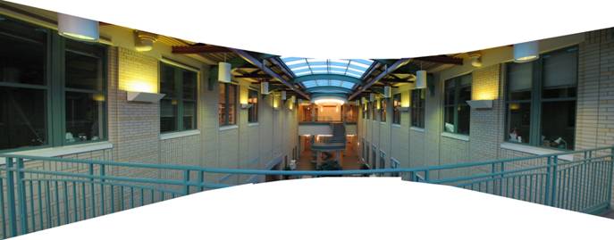
Good scenes are: building interiors with lots of detail, inside a canyon or forest, tall waterfalls, panoramas. The mosaic can extend horizontally, vertically, or can tile a sphere. You might want to shoot several such image sets and choose the best.

Shoot and digitize your pictures early - leave time to re-shoot in case they don't come out! Print and lay out your photos on a table to see approximately what the mosaic will look like.

Recover Homographies

Before you can warp your images into alignment, you need to recover the parameters of the transformation between each pair of images. In our case, the transformation is a homography: p’=Hp, where H is a 3x3 matrix with 8 degrees of freedom (lower right corner is a scaling factor and can be set to 1). One way to recover the homography is via a set of (p’,p) pairs of corresponding points taken from the two images . You will need to write a function of the form:

H = computeH(im1_pts,im2_pts)

where im1_pts and im2_pts are n-by-2 matrices holding the (x,y) locations of n point correspondences from the two images and H is the recovered 3x3 homography matrix. In order to compute the entries in the matrix H, you will need to set up a linear system of n equations (i.e. a matrix equation of the form Ah=b where h is a vector holding the 8 unknown entries of H). If n=4, the system can be solved using a standard technique. However, with only four points, the homography recovery will be very unstable and prone to noise. Therefore more than 4 correspondences should be provided producing an overdetermined system which should be solved using least-squares. In Matlab, both operations can be performed using the “\” operator (see help mldivide for details).

Establishing point correspondences is a tricky business. An error of a couple of pixels can produce huge changes in the recovered homography. The typical way of providing point matches is with a mouse-clicking interface. You can write your own using the bare-bones ginput function. Or you can use a nifty (but often flaky) cpselect. After defining the correspondences by hand, it’s often useful to fine-tune them automatically. This can be done by SSD or normalized-correlation matching of the patches surrounding the clicked points in the two images (see cpcorr), although sometimes it can produce undesirable results.

Warp the Images

Now that you know the parameters of the homography, you need to warp your images using this homography. Write a function of the form:

imwarped = warpImage(im,H)

where im is the input image to be warped and H is the homography. You can use either forward of inverse warping (but remember that for inverse warping you will need to compute H in the right “direction”). You will need to avoid aliasing when resampling the image. Consider using interp2, and see if you can write the whole function without any loops, Matlab-style. One thing you need to pay attention to is the size of the resulting image (you can predict the bounding box by piping the four corners of the image through H, or use extra input parameters). Also pay attention to how you mark pixels which don’t have any values. Consider using an alpha mask (or alpha channel) here.

Image Rectification

Once you get this far, you should be able to “rectify” an image. Take a few sample images with some planar surfaces, and warp them so that the plane is frontal-parallel (e.g. the night street examples above). You should do this before proceeding further to make sure your homography/warping is working. Note that since here you only have one image and need to compute a homography for, say, ground plane rectification (rotating the camera to point downward), you will need to define the correspondences using something you know about the image. E.g. if you know that the tiles on the floor are square, you can click on the four corners of a tile and store them in im1_pts while im2_pts you define by hand to be a square, e.g. [0 0; 0 1; 1 0; 1 1].

Blend the images into a mosaic

Warp the images so they're registered and create an image mosaic. Instead of having one picture overwrite the other, which would lead to strong edge artifacts, use weighted averaging. You can leave one image unwarped and warp the other image(s) into its projection, or you can warp all images into a new projection. Likewise, you can either warp all the images at once in one shot, or add them one by one, slowly growing your mosaic.

If you choose the one-shot procedure, you should probably first determine the size of your final mosaic and then warp all your images into that size. That way you will have a stack of images together defining the mosaic. Now you need to blend them together to produce a single image. If you used an alpha channel, you can apply simple feathering (weighted averaging) at every pixel. Setting alpha for each image takes some thought. One suggestion is to set it to 1 at the center of each (unwarped) image and make it fall off linearly until it hits 0 at the edges (or use the distance transform bwdist). However, this can produce some strange wedge-like artifacts. You can try minimizing these by using a more sophisticated blending technique, such as a Laplacian pyramid. If your only problem is “ghosting” of high-frequency terms, then a 2-level pyramid should be enough.

If your mosaic spans more than 180 degrees, you'll need to break it into pieces, or else use non-projective mappings, e.g. spherical or cylindrical projection.

At least one of your mosaics must be from outside the CMU campus. Climb the Cathedral of Learning! Hike through Schenley Park!

Submit Your Results

You will need to submit all your code as well as a webpage. Please remember to include a README with your code, describing where the various functions take place.

Bells & Whistles

• Your own ideas (N points): Be creative!
• Blending and Compositing (5 points each): Use homographies to combine images (or images and video) in interesting and creative ways. Here are a few suggestions:
• Put fake graffiti on buildings or chalk drawings on the ground
• Replace a road sign with your family portrait
• Project a movie onto a building wall
• Create a mosaic by spatially blending images taken at different times (day vs. night) or during different seasons
• Create a mosaic by spatially blending a historic photograph with a modern picture of the same place
• Create an interesting/bizarre mosaic, like the ones with multiple copies of the sample person…
• etc.
• Better blending (15 points): Implement multi-scale Laplacian pyramid blending. Compare it with just a two-level pyramid.
• Spherical/Cylindrical/polar mapping (10 points): Instead of projecting your mosaic onto a plane, try using another surface, such as a sphere or a cylinder. This is often a better way to represent really wide mosaics. Be clever: do the inverse sampling from the original pre-warped images to make your mosaic the best possible resolution. Pick the focal length (radius) that looks good.
• Use 3D rotational model (15 points): If your mosaic is a rotation about the same point and you don’t change zoom, you can use a simpler rotation-only transformation, which is more robust and requires less correspondences. This approach should also in theory help you find the focal length of your camera.
• 360 Cylindrical panorama (30 points): Instead of a planar-projection mosaic, do a cylindrical projection instead. Perform a cylindrical warp on all your input images and stitch them together using translation only. This is one way to produce a full 360 degree panorama (you can use a nifty Live Picture Viewer to display your panorama!). The down side is that this method places more requirements on your camera (you need to know the focal length and radial distortion coefficients), and your data (the images have to be exactly horizontal – use a tripod).
• Video mosaics (20 points): Capture two (or more) stationary videos (either from the same point, or of a planar/far-away scene). Compute homography and produce a video mosaic. You will need to worry about video synchronization (not too hard – a single parameter search). Also make sure that you shoot something where things are happening over short periods of time – video data gets really big really quickly. A good example would be capturing a football game from the sides of the stadium.

Appendix

Video Processing: Processing video in Matlab is a bit tricky. Theoretically, there is aviread but, under linux, it will only ready uncompressed AVIs. Most current digital cameras produce video in DV AVI format. One way to deal with this is to splice up the video into individual frames and then read them into Matlab one by one. On the graphics cluster, you can do (some variant of) the following to produce the frames from a video:

mplayer -vo jpeg -jpeg quality=100 -fps 30 mymovie.avi

Also note that handling video is a time-consuming thing (not just for you, but for the computer as well). If you shoot a minute of video, that’s already 60*30=1800 images! So, start early and don’t be afraid to let Matlab crunch numbers overnight.

Extracting camera parameters: For producing cylindrical or spherical mosaics, you will need to know more about your camera. The most important thing to know is the focal length f (in pixels, not mm). One way to obtain an educated guess about this value is to use the EXIF data field associated with images produced by most digital cameras. There are several programs for extracting EXIF data from a JPG image, such as this one. EXIF’s FocalLength gives you focal length in mm, so you will also need to know the pixel density (see FocalPlaneXResolution and FocalPlaneYResolution, but it’s usually in inches). Here is a handy calculator to help you figure out the right values. Note that this is only an estimate (in reality, due to different lenses, etc each particular camera (even of the same model!) will have slightly different parameters. For another, very applied, method called “Book and a Box”, check out Brett Allen’s solution for a similar assignment at UW.

Besides the focal length, other useful things to know are the optical center of the camera (for nothing better, assume it’s at the center of the image), and the distortion coefficients of the lens, k1 and k2. As a very simple hack, take a picture with lots of straight lines, hold k2=0 and try to find k1 that makes the lines in the image straight.