In Project 2, we both implemented face morphing. (Matt's work, Ben's work) However, in that project we limited ourselves to simple linear interpolations between the control points and color values of two images. Also, while it is possible to use the methods in Project 2 to "over-morph" someone to create a caricature, the caricatures produced are not as good as they could be, since they do not interpolate over actual facial features.
Thus, we set out to find and implement a superior face morphing method, armed with Matlab and a small face database from the Active Appearance Models website at DTU. We settled upon some of the techniques described in "Active Appearance Models" (Cootes '98).
The general idea is to use principal component analysis (PCA) to recover a facial coordinate space in order to make more meaningful morphs and caricatures. First we average the location of the control points for all faces to obtain an approximation for the average shape of a person. Next we form a triangulation of the average control points and then apply that triangulation to the control points of all of the source images. Based upon these triangulations, we can then compute the shape transformations from all of the source faces to the average, and warp the images to the average shape. Then we can perform a PCA on the intensity values of the colors of the warped input images to compute the color eigenvalues of the image set. Additionally we perform a PCA on the shape distortions between the base images and their average warps to get the eigenvalues for face shape. Now that we have both appearance coordinates and shape coordinates, we can interpolate through them to perform better-looking morphs. In addition, we can exaggerate a person's features by scaling out their vector in shape space.
If that doesn't make a lot of sense, read on for a detailed explanation of how it all works, and what can be done.
Simply put, Principal Component Analysis is a process whereby a data set expressed in M-dimensional space is reduced to a K dimensional space, where the K dimensions computed represent the K-axis subspace of the original data set which accounts for as much of the variation in the data set as possible (and thus are optimal for moving about the given data set in K dimensions).
PCA is necessary to this application because an image of a face with pixel dimensions (W x H) has W*H degrees of freedom (every pixel can vary its color independent of every other). Thus without PCA, for the 400x480 images we used in this project, calculations in 192,000 dimensional space would be required. This, naturally, is computationally unreasonable. By using PCA, this 192,000 dimensional space can be reduced to an arbitrarily small (and therefore much more tractable) coordinate space, with each of the resulting axes expressing the most important aspects of face-ness (thus the term principal component analysis).
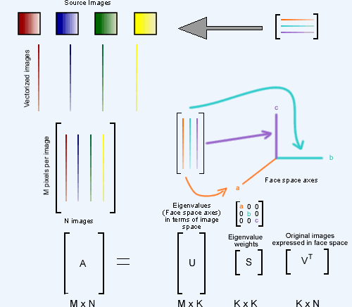
PCA is done by performing singular value decomposition upon the given data set. This generates a set of three matrices, U, S, and V.
U is an MxK matrix. The columns of U are a list of normalized eigenvalues representing the axes of greatest change, in terms of the 192,000 dimensions of 400x480 image space. Essentially a conversion guide, where each column of the matrix represents one particular eigenvalue's magnitudes in image space.
S is a KxK, diagonal matrix. The values on the diagonals represent the weights for each of the eigenvalues in matrix U. This matrix allows us to rank the eigenvalues in order of importance (a larger weight equals a greater importance).
V is a KxN matrix. The columns of this matrix give the representation of the original 192,000 dimensional image inputs in terms of the new coordinate space of the eigenvalues.
The critical relation between these matrices is shown above:
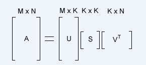
This allows us to take novel images (expressed in the same 400x480 image space) and manipulate them in our face space. We start with our known image A, and neither U nor S change based upon the given image (so long as the image is in the same image space for which U and S were calculated), thus manipulating an image in our eigen-space is merely a matter of solving for V.
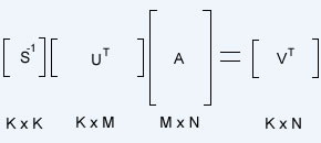
Since U is orthonormal (eigenvalues are orthogonal and the columns of U are normalized), the inverse of U is equal to its transpose. S is square and easily invertable on its own, thus we have our equation for V
Below are the top 15 appearance eigenvalues for our 40 face pool.
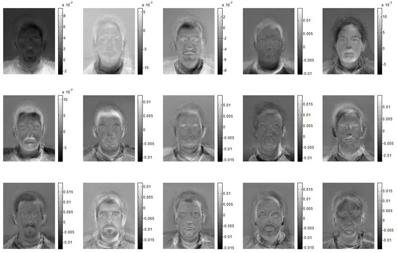
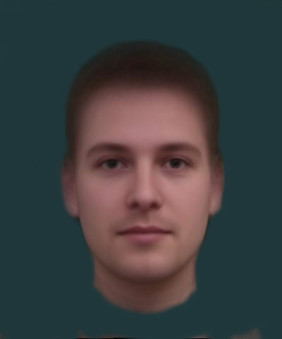
Each eigenvalue of this face space represents some aspect of face-ness. Before we move on to make caricatures by magnifying the differences between people and the average face, which involves relative magnification of a person's variance from the average face, we wish to examine exactly what it is some of our facial axes represent. The average face we computed based on our initial 40 faces is shown below. It is both the average shape and color (and has been touched up a bit in Photoshop to remove non-face regions).
We created five animations which display the effects of translating along the axes specified by the top five shape eigenvalues. These images are each centered around the average face, since it is the origin of face space. They begin at a negative point along the given face axis, move through the origin, and stop an equal distance into the positive space of the particular axis. The coordinate value of all other axes is 0 throughout the entire animation- movement occurs only on the given axes. The choice for the specific values over which to iterate each axis was made by a trial and error process. This was necessary since face space coordinates are in a completely foreign coordinate space with no clear semantic relation.
Translation along facial axis 1 (values range from -1.0 to 1.0)
Translation along facial axis 2 (values range from -1.5 to 1.5)
Translation along facial axis 3 (values range from -1.0 to 1.0)
Translation along facial axis 4 (values range from -2.0 to 2.0)
Translation along facial axis 5 (values range from -1.5 to 1.5)
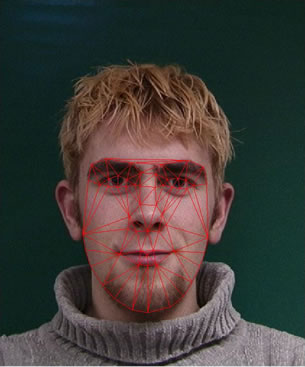
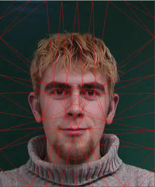
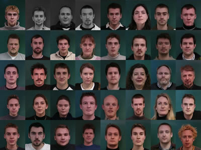
As we previously mentioned, we used a small face database from the Active Appearance Models website at DTU for our main face source. These faces were all marked in the same way with 58 control points (shown in red below on the left). Then, using all 40 of our source images, we averaged the control points to compute the average face shape (The blue dots on the right image below).

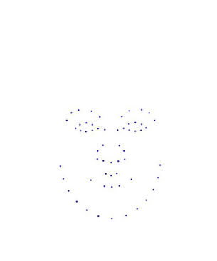
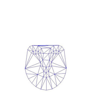
Once the average control point set (face shape) was obtained, a triangulation of this average (a mapping of control points into triangles) was computed, and then applied to the source images.
From here we had all of the data necessary to launch our algorithm.
However, the data set was not without issues. The choice of the positioning of the control points, at least for our purposes, left something to be desired. There were no control points marking the outline of the face except for the chin. This completely discounted some facial features, such as the ears, size of forehead, and hairline. As a result, triangle meshes of the images had extremely poor detail in these areas, producing smearing artifacts due to an inability to finely control those areas. Also, the lack of control points anywhere not in the center of the face left us with basically a naive crossfade between image regions not contained within the central face region. To obviate this problem, we added a border of control points along the edges of the image, every 10% of the way. This gave the warping process much needed flexibility and drastically reduced (though did not eliminate in all cases) the problem.
Another major problem with the data set was the variation in face location and size between images, as seen below.
This causes the computed face space to become polluted with false facial differences caused by camera position and zoom, instead of only computing true face variance. The overall result of this turned out to be a barrel distortion effect on the images, and the first eigenvalue returned from these images was the degree of the barrel distortion. We corrected this by attempting to apply a rough recentering heuristic. Our solution assumed that the distance between the eyes of any individual was constant, and used that as a metric to re-align the images. We averaged the 8 control points around the each eye to compute a basic "eye position," and then used the eye positions of each source image against the eye position of the average image to compute a linear-conformal (2D translation, rotation, and/or scaling) transformation. We apply this transformation to the control points of the image for the purposes of PCA calculations and interpolation. As a final step we reverse the transformation to return the face to its normal scale and orientation. However, once again the lack of control points outside of the inner regions of the face causes distortion around the non-face portion of the image during this process.
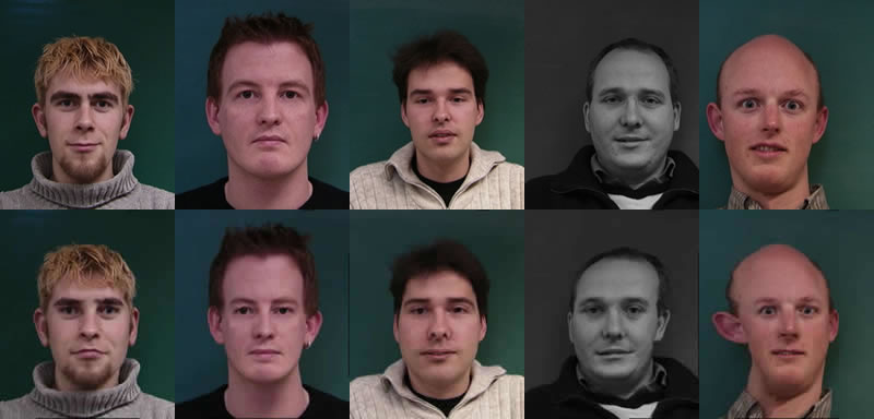
The basic input images are on the top row, the corrected images are on the bottom row.
Once we have recovered our new face space, making caricatures of people is surprisingly easy. In face space, we can compute the deviation of a given person from the average face. This is simple since we had subtracted out the average face before PCA, so the face space vector is the same as the difference between an individual face and the average. This vector is the essence of that person, and we can scale that vector outward or inward to make a person more or less like themselves. There is a limit to how far the caricature vector can be pushed though, as the triangle mesh will begin to break down at a certain point.
Something to consider, though, is how many of the eigenvalues of the face space to use. If too many or all of the eigenvalues are used, then the results are nearly or completely identical to that of linear interpolation. If too few of the eigenvalues are used, then too much of the individuality is lost during the transformations and they become oversimplified.
Thus, in the interest of seeing exactly what tweaking with these parameters does, for all of our faces we computed caricatures over a variety of caricature vector scaling factors (1.0, 2.0, 2.5, 3.0), and for multiple numbers of eigenvalues (5, 10, 15, all (linear interpolation)). Click on the thumbnail below to browse our gallery of results. Note: When attempting to compute 15 eigenvalue caricatures at a 3.0 scaling of the caricature vector, in almost every case Matlab returned error.
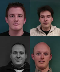
At least in theory, we should be able to input any new face that has been marked up with control points in the same way as our initial faces. This is because all faces should be representable as a point in our face space. Their point can then be manipulated into caricatures exactly the same way the previous faces were. We tried this on the pictures of people from our class that had been taken for Project 2. Each picture below is a pair with the original on top, and the level 2.0 caricature on bottom.
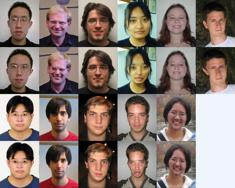
We had varied success with this approach. The faces we used varied in angle, scale, and facial expression quite a bit, and the set of control points we were using could not adequately handle those deviations. This led to some rather unpleasant results when the caricatures began compensating for smiles or tilted heads.
We also constructed an animation of the caricaturization process of one of our subjects, simply as a point of interest. In this animation the subject progresses from his normal face (a 1.0 scaling factor applied to his face space vector), to a 5.0 scaling factor. Note that the progression of the subject in this image is through the subject's representation in facial coordinate space, and not simply a linear interpolation around the image plane.
Morphing faces is a simple process once the face space and the appearance space have been found. Instead of linearly interpolating control points or pixel values, we interpolate their face space vectors, and then reconstruct the images from those vectors. We produced some movies of morphing between faces in our initial set. It should be possible to morph in new faces, the same way we added new faces for the caricatures, too. We ran into two main problems when computing the face morph. The first was that, since each point in image space has a number of coordinates equal to the number of pixels (for each color plane), we had to reduce the images to grayscale to keep from running out of memory in Matlab. The second was that when using reduced numbers of eigenvectors to represent our appearance space, faces were not reconstructed exactly. The movies below illustrate this. The first uses only 15 eigenvectors to describe all the pixels in the image, and therefore the faces are not as distinct. Later movies used 30 eigenvectors, and the resemblance to their original is much stronger. We think these morphs are much smoother, both in shape and color, to the ones we computed in Project 2.
Morphing between two faces (5 shape eigenvectors, 15 appearance eigenvectors)
Morphing between the same two faces (5 shape eigenvectors, 30 appearance eigenvectors)
Morphing between two very different faces (10 shape eigenvectors, 30 appearance eigenvectors)